Quick start guide
Contents
Quick start guide#
Install Lakeview#
Install Lakeview from PyPI:
pip install lakeview
Import Lakeview#
import lakeview as lv
Get the BAM file#
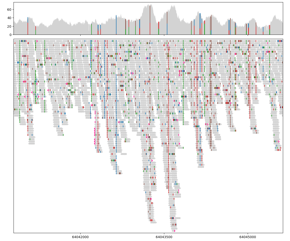
Wwe are going to visualize Illumina paired-end sequencing data from the SKBR3 breast cancer cell line. This example dataset is also used by IGV Web. Another example based on the same dataset can be found in Gallery.
Here assume the BAM file to be visualised is available locally. If the BAM file exists on a remote server instead of your local machine, you may choose to:
download the entire BAM file to your local machine;
download a subset of the BAM file that contains your region of interest;
or run Lakeview on the server and download the output figures.
BAM_PATH = "../../tests/data/SKBR3_Illumina_550bp_pcrFREE.bam"
Load data from the BAM file#
Lakeview works by first loading the alignment data into the memory before making visualisations, which enables the data to be checked and optionally preprocessed before visualisation. If you are running Python interactively (e.g. via Jupyter Notebook), you will also be able to make incremental adjustments to the plot without reloading the data.
# Specify the region of interest as "chromosome:start-end".
# Commas are optional.
REGION = "17:64,040,802-64,045,633"

# Load data from the BAM file
painter = lv.SequenceAlignment.from_file(BAM_PATH, region=REGION)
Create an empty GenomeViewer#
A GenomeViewer represents a blank canvas with one or more tracks, all of which share the same start and end coordinates. It handles general operations related to the visualisation, such as creating/saving the figure, specifying the figure size, adjusting start/end coordinates, labelling tracks, setting a title, and formatting ticks.
If you are familiar with Matplotlib, think of GenomeViewer as a wrapper around a Figure with several tracks (Axes) that share the x axis limits.
# Create a GenomeViewer with two tracks
gv = lv.GenomeViewer(tracks=2, height_ratios=(1, 6), figsize=(12, 10))
Show code cell output

# Display the (currently empty) figure
gv.figure

Plot alignment data#
The SequenceAlignment class has two methods for plotting: draw_pileup and draw_alignment. These methods draw the visualisation on the given track (Axes), and are the main entrance point for further customisation.
# Draw alignment pileup in the first track
painter.draw_pileup(gv.axes[0])

# Draw aligned segments in the second track
painter.draw_alignment(gv.axes[1])

# Adjust start/end coordinates
gv.set_xlim(64040802, 64045633)
(64040802.0, 64045633.0)
# Display the (now painted) figure
gv.figure

Save the output figure#
The output figure can be saved in various bitmap and vector formats, such as PNG, JPEG, PDF, SVG and EPS.
# Save the figure as a PNG graphic with resolution 300 dots per inch (DPI)
gv.savefig("SKBR3.png", dpi=300)